Note
This is the documentation for the current state of the development branch of rustworkx. The documentation or APIs here can change prior to being released.
Introduction to rustworkx#
The rustworkx library is a Python library for working with graphs (or networks) and graph theory.
This guide serves as an introduction to working with rustworkx. If you’re a current or past NetworkX user who is looking at using rustworkx as a replacement for NetworkX, you can also refer to rustworkx for NetworkX users for a detailed comparison.
Installing rustworkx#
To install rustworkx you need a Python installation. Rustworkx works in any Python environment. If you already have Python, you can install rustworkx with:
pip install rustworkx
(if you’re running on a supported platform, if you’re not you will need to refer to the Installing on a platform without precompiled binaries on how to build and install)
How to import rustworkx#
To access rustworkx and its functions import it into your Python code like this:
import rustworkx as rx
We shorten the name to rx for better readability of code using Rustworkx.
This is a widely adopted convention that you can follow.
Creating a Graph#
To create an empty undirected graph
G = rx.PyGraph()
A PyGraph is comprised of nodes (vertices)
and unordered pairings of nodes (called edges, links, etc). Both nodes and
edges in rustworkx have an assigned data payload (also referred to as a weight
in the API and documentation) which can be any Python object (e.g. a numeric
value, a string, an image, an XML object, another graph, a custom node object,
etc.). Nodes and edges are uniquely identified by an integer index
which is stable for the lifetime of that node or edge in the graph. These
indices are not guaranteed to be contiguous as removed nodes or
edges will leave holes in the sequence of assigned indices, and an index
can be reused after a removal.
Nodes#
The graph
To get started we can add a single node:
G.add_node(1)
0
The add_node() method returns an integer. This integer
is the index used to uniquely identify this new node in the graph. You can use
this index to identify the node as long as node remains in the graph.
It is also possible to add nodes to
indices = G.add_nodes_from(range(5))
print(indices)
NodeIndices[1, 2, 3, 4, 5]
Just as with add_node(), the
add_nodes_from() method returns the indices for the nodes
added as a NodeIndices object, which is a custom sequence
type that contains the index of each node in the order it’s added from the input
sequence.
In the above cases, we were adding nodes with a data payload of type integer (e.g. G.add_node(1)).
However, rustworkx doesn’t place constraints on what the node data payload can
be, so you can use more involved objects including types which are not
hashable. For
example, we can add a node with a data payload that’s a
dict:
G.add_node({
    "color": "green",
    "size": 42,
})
6
A discussion of how to select what to use for your data payload is in the What to use for node and edge data payload section.
Edges#
The graph
G.add_edge(1, 2, None)
0
This will add an edge between node index 1 and node index 2 with a
data payload of None. Similarly to add_node(), the
add_edge() method returns the new edge’s unique
index.
Examining elements of a graph#
We can examine the nodes and edges of a graph in rustworkx fairly easily. The
first thing to do is to get a list of node and edge indices using
node_indices() and
edge_indices():
node_indices = G.node_indices()
edge_indices = G.edge_indices()
print(node_indices)
print(edge_indices)
NodeIndices[0, 1, 2, 3, 4, 5, 6]
EdgeIndices[0]
Since indices are the unique identifiers for nodes and edges, they’re your
handle to elements in the graph. This is especially important for edges in the
multigraph case, or where you have identical data payloads between multiple
nodes. You can use the indices to access the data payload. For nodes, the
PyGraph object behaves like a
mapping with the
index:
first_index_data = G[node_indices[0]]
print(first_index_data)
1
For edges, you can use the get_edge_data_by_index()
method to access the data payload for a given edge and
get_edge_endpoints_by_index() to get the endpoints
of a given edge from its index:
first_index_data = G.get_edge_data_by_index(edge_indices[0])
first_index_edgepoints = G.get_edge_endpoints_by_index(edge_indices[0])
print(first_index_edgepoints)
print(first_index_data)
(1, 2)
None
We don’t implement the mapping protocol for edges, so there is a helper
method available to get the mapping of edge indices to edge endpoints and
data payloads, edge_index_map():
print(G.edge_index_map())
EdgeIndexMap{0: (1, 2, None)}
Additionally, you can access the list of node and edge data payloads directly
with nodes() and edges()
print("Node data payloads")
print(G.nodes())
print("Edge data payloads")
print(G.edges())
Node data payloads
[1, 0, 1, 2, 3, 4, {'color': 'green', 'size': 42}]
Edge data payloads
[None]
Removing elements from a graph#
You can remove a node or edge from a graph in a similar manner to adding
elements to the graph. There are methods remove_node(),
remove_nodes_from(),
remove_edge(),
remove_edge_from_index(), and
remove_edges_from() to remove nodes and edges from
the graph. One thing to note is that removals can introduce holes in the
lists of indices for nodes and edges in the graph. For example:
graph = rx.PyGraph()
graph.add_nodes_from(list(range(5)))
graph.add_nodes_from(list(range(2)))
graph.remove_node(2)
print(graph.node_indices())
NodeIndices[0, 1, 3, 4, 5, 6]
You can see here that 2 is now absent from the node indices of graph.
Also, after a removal, the index of the removed node or edge will be reused on
subsequent additions. For example, building off the previous example if you ran
graph.add_node("New Node")
2
this new node is assigned index 2 again.
Modifying elements of a graph#
The graph classes in rustworkx also allow for in place mutation of the payloads for elements in the graph. For nodes you can simply use the mapping protocol to change the payload via its node index. For example:
last_index = graph.node_indices()[-1]
graph[last_index] = "New Payload"
print(graph[last_index])
New Payload
You can update the payload of any node in the graph using this interface. For
edges you can leverage the update_edge or
update_edge_by_index methods to update an edge’s payload
in place. For example:
edge_index = graph.add_edge(0, 1, None)
graph.update_edge_by_index(edge_index, "New Edge Payload")
print(graph.get_edge_data_by_index(edge_index))
New Edge Payload
What to use for node and edge data payload#
In the above examples for the most part we use integers, strings, and None
for the data payload of nodes and edges in graphs (mostly for simplicity).
However, rustworkx allows the use of any Python object as the data payload for
nodes and edges. This flexibility is very powerful as
it allows you to create graphs that contain other graphs, graphs that contain
files, graphs with functions, etc. This means you only need to keep a reference
to the integer index returned by rustworkx for the objects you use as a data
payloads to find those objects in the graph. For example, one approach you can
take is to store the index as an attribute on the object you add to the graph:
class GraphNode:

    def __init__(self, value):
        self.value = value
        self.index = None

graph = rx.PyGraph()
index = graph.add_node(GraphNode("A"))
graph[index].index = index
Additionally, at any time you can find the index mapping to the data payload and build a mapping or update a reference to it. For example, building on the above example you can update the index references all at once after creation:
class GraphNode:
    def __init__(self, value):
        self.index = None
        self.value = value

    def __str__(self):
        return f"GraphNode: {self.value} @ index: {self.index}"

class GraphEdge:
    def __init__(self, value):
        self.index = None
        self.value = value

    def __str__(self):
        return f"EdgeNode: {self.value} @ index: {self.index}"

graph = rx.PyGraph()
graph.add_nodes_from([GraphNode(i) for i in range(5)])
graph.add_edges_from([(i, i + 1, GraphEdge(i)) for i in range(4)])
# Populate index attribute in GraphNode objects
for index in graph.node_indices():
    graph[index].index = index
# Populate index attribute in GraphEdge objects
for index, data in graph.edge_index_map().items():
    data[2].index = index
print("Nodes:")
for node in graph.nodes():
    print(node)
print("Edges:")
for edge in graph.edges():
    print(edge)
Nodes:
GraphNode: 0 @ index: 0
GraphNode: 1 @ index: 1
GraphNode: 2 @ index: 2
GraphNode: 3 @ index: 3
GraphNode: 4 @ index: 4
Edges:
EdgeNode: 0 @ index: 0
EdgeNode: 1 @ index: 1
EdgeNode: 2 @ index: 2
EdgeNode: 3 @ index: 3
Accessing edges and neighbors#
You can access edges from a node using the incident_edges()
method:
print(G.incident_edges(2))
EdgeIndices[0]
which will return the edge indices of the edges incident to node 2. You
can also find the neighbor nodes using the neighbors()
method:
print(G.neighbors(2))
NodeIndices[1]
which returns the node indices of any neighbors of node 2.
Graph Attributes#
Graphs in rustworkx have an attribute which can be used to assign
metadata to a graph object. This can be assigned at object creation or
accessed and modified after creation with the attrs attribute.
This attribute can be any Python object and defaults to being None if not
specified at graph object creation time. For example:
graph = rx.PyGraph(attrs=dict(day="Friday"))
graph.attrs['day'] = "Monday"
Or, you could use a custom class like:
class Day:

    def __init__(self, day):
        self.day = day

graph = rx.PyGraph(attrs=Day("Friday"))
graph.attrs = Day("Monday")
Directed Graphs#
A directed graph is a graph that is made up of a set of nodes connected by
directed edges (often called arcs). Edges have a directionality which is
different from undirected graphs where edges have no notion of a direction to
them. In rustworkx the PyDiGraph class is used to create
directed graphs. For example:
from rustworkx.visualization import mpl_draw

path_graph = rx.generators.directed_path_graph(5)
mpl_draw(path_graph)
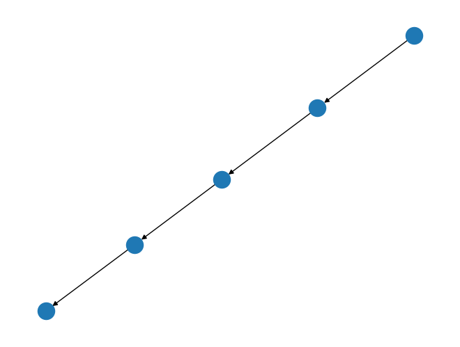
In this example we created a directed path graph with 5 nodes. This shows the directionality of the edges in the graph visualization with the arrow head pointing to the target node.
Multigraphs#
By default all graphs in rustworkx are multigraphs. This means that each
graph object can contain parallel edges between nodes. However, you can set
the multigraph argument to False on the PyGraph and
PyDiGraph constructors when creating a new graph object to
prevent parallel edges from being introduced. When multigraph is set to False
any method call made that would add a parallel edge will instead update the
existing edge’s weight/data payload. For example:
graph = rx.PyGraph(multigraph=False)
graph.add_nodes_from(range(3))
graph.add_edges_from([(0, 1, 'A'), (0, 1, 'B'), (1, 2, 'C')])
mpl_draw(graph, with_labels=True, edge_labels=str)
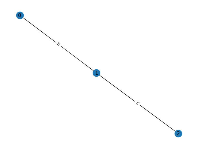
In this example, our attempt to add a parallel edge between nodes 0
and 1 will instead result in the existing edge’s data payload being updated from
'A' to 'B'.
Graph Generators and operations#
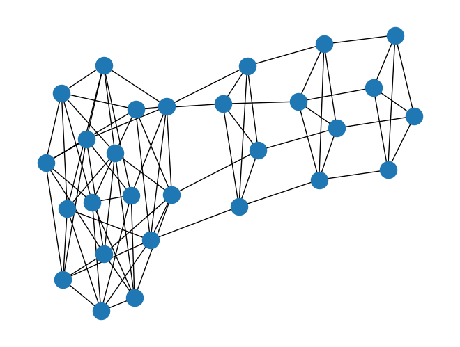
In addition to constructing graphs one node and edge at a time, you can also create graphs using the Generators, Random Graph Generator Functions, and Graph Operations to quickly generate graphs and/or apply different operations on the graph. For example:
lolipop_graph = rx.generators.lollipop_graph(4, 3)
mesh_graph = rx.generators.mesh_graph(4)
combined_graph = rx.cartesian_product(lolipop_graph, mesh_graph)[0]
mpl_draw(combined_graph)
Additionally there are alternate constructors such as
read_edge_list() or from_adjacency_matrix()
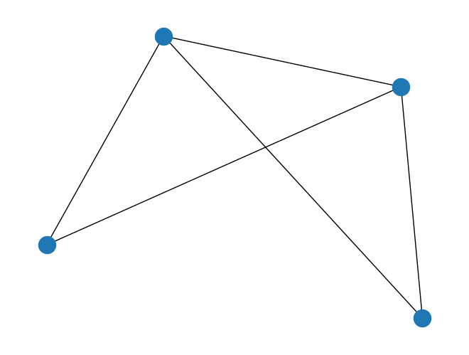
for building graphs from files or other inputs. For example:
import tempfile

with tempfile.NamedTemporaryFile('wt') as fd:
    path = fd.name
    fd.write('0 1\n')
    fd.write('0 2\n')
    fd.write('0 3\n')
    fd.write('1 2\n')
    fd.write('2 3\n')
    fd.flush()
    graph = rx.PyGraph.read_edge_list(path)
mpl_draw(graph)
Analyzing graphs#
The structure of a graph
G = rx.PyGraph()
G.extend_from_edge_list([(0, 1), (0, 2)])
new_node = G.add_node("spam")
print(rx.connected_components(G))
degrees = {}
for node in G.node_indices():
    degrees[node] = G.degree(node)
print(degrees)
[{0, 1, 2}, {3}]
{0: 2, 1: 1, 2: 1, 3: 0}
G.remove_node(new_node)
G.extend_from_edge_list([(0, 3), (0, 4), (1, 2)])
rx.transitivity(G)
0.375
See the Algorithm Functions API documentation section for a list of the available functions and corresponding usage information.
Drawing graphs#
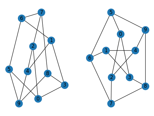
There are two visualization functions provided in rustworkx for visualizing
graphs. The first is mpl_draw(), which uses the
matplotlib library to render the
visualization of the graph. The mpl_draw()
function relies on the Layout Functions provided with rustworkx to
generate a layout (the coordinates to draw the nodes of the graph) for the
graph (by default spring_layout() is used). For example:
import matplotlib.pyplot as plt

G = rx.generators.generalized_petersen_graph(5, 2)
subax1 = plt.subplot(121)
mpl_draw(G, with_labels=True, ax=subax1)
subax2 = plt.subplot(122)
layout = rx.shell_layout(G, nlist=[[0, 1, 2, 3, 4], [6, 7, 8, 9, 5]])
mpl_draw(G, pos=layout, with_labels=True, ax=subax2)
The second function is graphviz_draw(), which
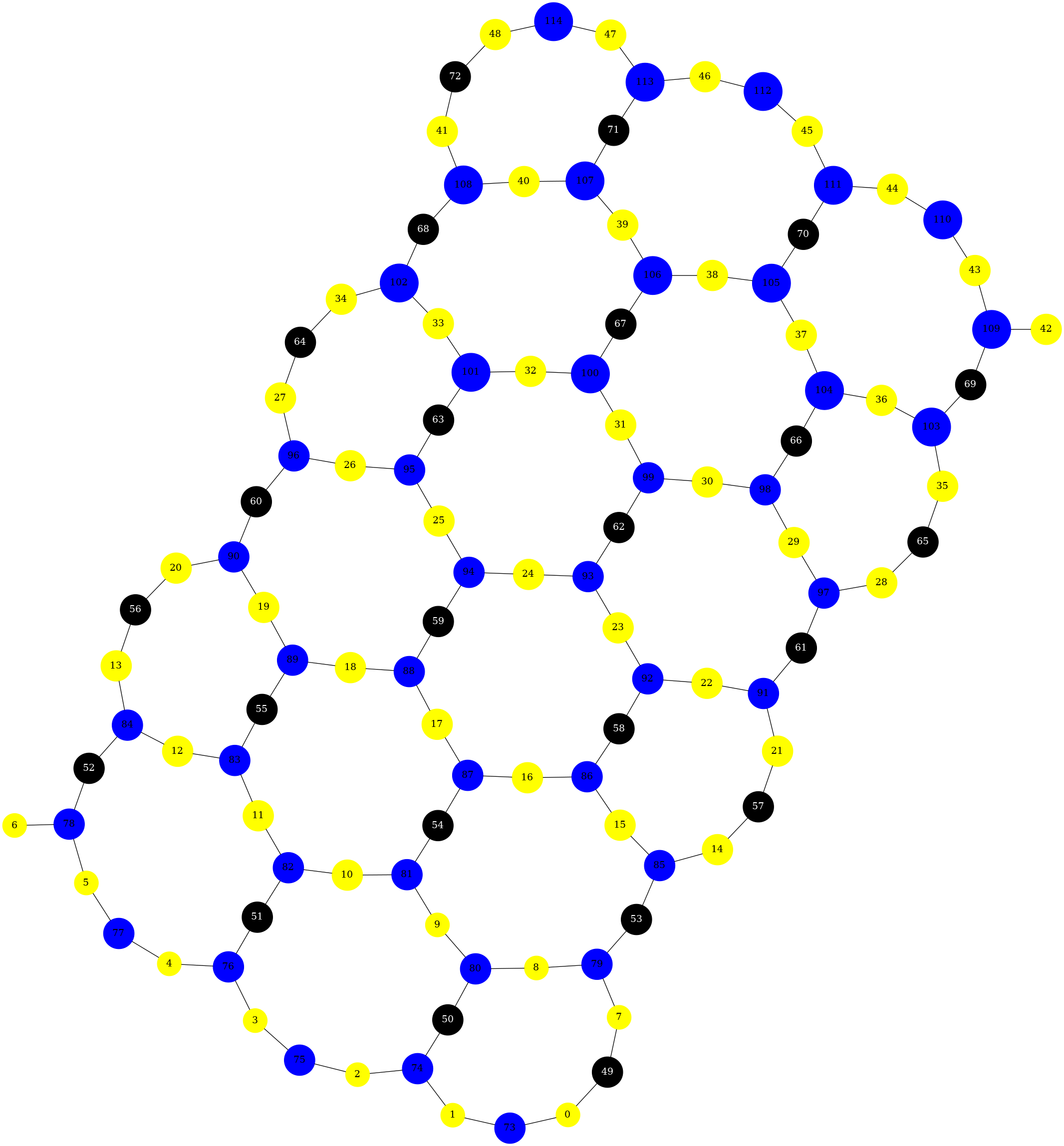
uses Graphviz to generate visualizations. For
example:
from rustworkx.visualization import graphviz_draw

G = rx.generators.heavy_hex_graph(7)
# set data payload to index
for node in G.node_indices():
    G[node] = node

def node_attr_fn(node):
    attr_dict = {
        "style": "filled",
        "shape": "circle",
        "label": str(node)
    }
    # Data nodes are yellow
    if node < 7 * 7:
        attr_dict["color"] = "yellow"
        attr_dict["fill_color"] = "yellow"
    # Syndrome nodes are black
    elif node >= 7 * 7 and node < (7 * 7) + ((7 - 1) * (7 + 1) / 2):
        attr_dict["color"] = "black"
        attr_dict["fill_color"] = "black"
        attr_dict["fontcolor"] = "white"
    # Flag quits are blue
    else:
        attr_dict["color"] = "blue"
        attr_dict["fill_color"] = "blue"
    return attr_dict

graphviz_draw(G, node_attr_fn=node_attr_fn, method="neato")
Generally, when deciding which visualization function to use, there are a few
considerations to make. mpl_draw() is a better
choice for smaller graphs or cases where you want to integrate your graph
drawing as part of a larger visualization.
graphviz_draw() is typically a better choice
for larger graphs, because Graphviz is a dedicated tool for drawing graphs.