Note

This is the documentation for the current state of the development branch of rustworkx. The documentation or APIs here can change prior to being released.

Directed Acyclic Graphs

This tutorial will explore using rustworkx to work with directed acyclic graphs (also known as DAGs).

Directed Graph

As a primer, let’s first review the broader concept of a directed graph (without the acyclic restriction).

A directed graph is made up of a set of nodes connected by directed edges (often called arcs). Directed edges can only be followed in one direction, which is different from the edges found in undirected graphs, which can be followed in either direction. For example:

import rustworkx as rx
from rustworkx.visualization import mpl_draw

path_graph = rx.generators.directed_path_graph(5)
mpl_draw(path_graph)

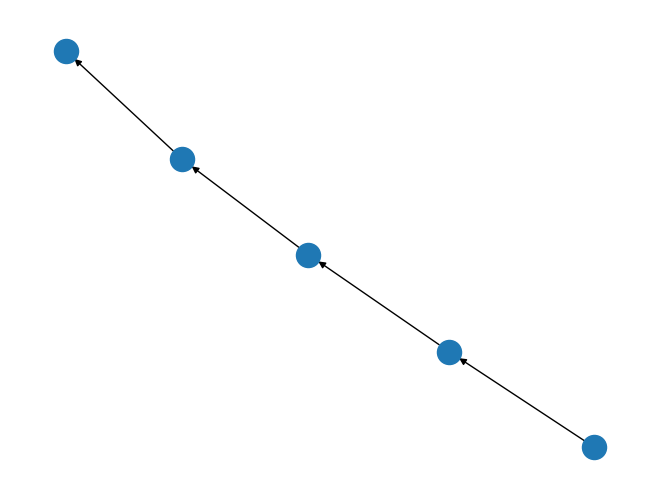
In this example, we’ve created a 5 node directed path graph. The directionality of each edge is denoted by the arrow head, which points to the target node. The node at the other end of the edge is called the source.

Directed Acyclic Graphs

A directed acyclic graph is a directed graph which also doesn’t contain any cycles. A cycle is a non-empty trail [1] in which the first and last nodes in the trail are the same. For example:

cycle_graph = rx.generators.directed_cycle_graph(5)
mpl_draw(cycle_graph)

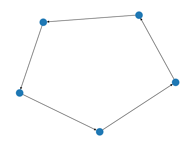
is not acyclic. While the earlier path graph is acyclic.

In rustworkx you can create a new PyDiGraph object that enforces that no cycle is added by using the check_cycle constructor property

dag = rx.PyDiGraph(check_cycle=True)

or after a PyDiGraph object is created with the check_cycle attribute:

dag.check_cycle = True

You can also check the status of cycle checking by inspecting the check_cycle attribute:

print(dag.check_cycle)

True

With check_cycle set to True, methods that add edges to the graph (e.g. PyDiGraph.add_edge()) will raise an error if a cycle would be introduced. This checking does come with a noticeable (and potentially large) runtime overhead so it’s best to only use it if it’s strictly necessary. You can also avoid this overhead by using PyDiGraph.add_parent() and PyDiGraph.add_child() as both add a new node and edge simultaneously and neither can introduce a cycle.

[1]

A trail is a sequence of nodes and edges on the graph where each edge is distinct in the walk.

Applications of DAGs

Task Scheduling

A topological sort of a directed acyclic graph defined as \(G = (V,E)\) is a linear ordering of all its nodes such that if \(G\) contains an edge \((u, v)\) then \(u\) appears before v. This only works with DAGs since a cycle in the graph \(G\) would make it impossible to find such a linear ordering.

A common application of DAGs is to use a topological sort to schedule a sequence of jobs or tasks based on their dependencies. Jobs are represented by nodes and an edge from node \(u\) to node \(v\) implies that job \(u\) must be completed before job \(v\). A topological sort of a directed acyclic graph will give an order in which to perform these jobs. For example:

from rustworkx.visualization import graphviz_draw

# Create a job dag
dependency_dag = rx.PyDiGraph(check_cycle=True)
job_a = dependency_dag.add_node("Job A")
job_b = dependency_dag.add_child(job_a, "Job B", None)
job_c = dependency_dag.add_child(job_b, "Job C", None)
job_d = dependency_dag.add_child(job_a, "Job D", None)
job_e = dependency_dag.add_parent(job_d, "Job E", None)
job_f = dependency_dag.add_child(job_e, "Job F", None)
dependency_dag.add_edge(job_a, job_f, None)
dependency_dag.add_edge(job_c, job_d, None)

graphviz_draw(dependency_dag, node_attr_fn=lambda node: {"label": str(node)})

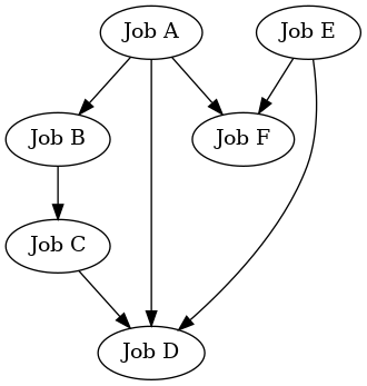
Above we define a DAG with 6 jobs and dependency relationship between these jobs. Now if we run the topological_sort() function on the graph it will return a linear order to execute the jobs that will respect the dependency relationship.

topo_sorted = rx.topological_sort(dependency_dag)
# Print job labels
print([dependency_dag[job_index] for job_index in topo_sorted])

['Job E', 'Job A', 'Job F', 'Job B', 'Job C', 'Job D']

Qiskit’s Compiler

Another application using directed acyclic graphs is the compiler in Qiskit. Qiskit is an SDK for working with quantum computing. Qiskit’s compiler internally represents a quantum circuit as a directed acyclic graph. Rustworkx was originally started to accelerate the performance of the Qiskit compiler’s use of directed acyclic graphs.

To examine how Qiskit uses DAGs, we first need to look at a quantum circuit. A quantum circuit is a computation routine consisting of coherent quantum operations on quantum data. It is an ordered sequence of quantum operations including gates, measurements and resets which may be conditioned on real-time classical computation. A quantum circuit is represented graphically like:

        ┌───┐      ░ ┌─┐
   q_0: ┤ H ├──■───░─┤M├───
        └───┘┌─┴─┐ ░ └╥┘┌─┐
   q_1: ─────┤ X ├─░──╫─┤M├
             └───┘ ░  ║ └╥┘
meas: 2/══════════════╩══╩═
                      0  1

The specifics of this circuit aren’t important here beyond the fact that we have 2 qubits, q_0 and q_1, 2 classical bits, c_0 and c_1, and a series of operations on those qubits with a dependency ordering. The last operation on each qubit is a measurement on q_0 that is stored in c_0 and q_1 that is stored in c_1.

We can represent this quantum circuit as a directed acyclic graph like Qiskit does internally with:

dag = rx.PyDiGraph()
# Input nodes:
in_nodes = dag.add_nodes_from(["q_0", "q_1", "c_0", "c_1"])
# Output nodes
out_nodes = dag.add_nodes_from(["q_0", "q_1", "c_0", "c_1"])
# Add H gate
h_gate = dag.add_child(in_nodes[0], "h", "q_0")
# Add CX Gate
cx_gate = dag.add_child(h_gate, "cx", "q_0")
dag.add_edge(in_nodes[1], cx_gate, "q_1")
# Add measure Gates
meas_q0 = dag.add_child(cx_gate, "measure", "q_0")
meas_q1 = dag.add_child(cx_gate, "measure", "q_1")
# Measure q0 instruction edges
dag.add_edge(meas_q0, out_nodes[0], "q_0")
dag.add_edge(in_nodes[2], meas_q0, "c_0")
dag.add_edge(meas_q0, out_nodes[2], "c_0")
# Measure q1 instruction edges
dag.add_edge(meas_q1, out_nodes[1], "q_1")
dag.add_edge(in_nodes[3], meas_q1, "c_1")
dag.add_edge(meas_q1, out_nodes[3], "c_1")

graphviz_draw(
    dag,
    node_attr_fn=lambda node: {"label": str(node)},
    edge_attr_fn=lambda edge: {"label": str(edge)}
)

In this representation of the circuit, the flow of data through the bits is modeled by edges. The first set of nodes are input nodes and the last set are output nodes representing the beginning state and end state of each bit (both classical and quantum). The compiler then runs analysis and transformations on the DAG representation of a quantum circuit to optimize the quantum circuit so it can be executed on real hardware. For example, a simple transformation pass is to translate the quantum gates in the circuit to the set of gates allowed on a device. If we were to attempt to run the above circuit on a QPU that didn’t natively support the H quantum gate, we’d first have to translate it to an equivalent series of instructions that the hardware actually supported. A simplified view of how this is performed is:

# Equivalency matrix
translation_matrix = {"h": ["rz(pi/2)", "sx", "rz(pi/2)"]}
# Insructions natively supported on target QPU
hardware_instructions = {"measure", "cx", "sx", "rz", "x"}

# Iterate over instructions in order and replace gates outside of native
# instruction set with a subcircuit from the translation matrix
for gate_index in rx.topological_sort(dag):
    if gate_index not in in_nodes and gate_index not in out_nodes:
        if dag[gate_index] not in hardware_instructions:
            edge_val = dag.out_edges(gate_index)[0][2]
            equivalent_subcircuit = rx.PyDiGraph()
            count = 0
            for node in translation_matrix[dag[gate_index]]:
                if count == 0:
                    equivalent_subcircuit.add_node(node)
                else:
                    equivalent_subcircuit.add_child(count - 1, node, edge_val)
                count += 1

            def map_fn(source, target, weight):
                if source == gate_index:
                    return len(equivalent_subcircuit) - 1
                else:
                    return 0

            dag.substitute_node_with_subgraph(
                gate_index,
                equivalent_subcircuit,
                map_fn
            )

graphviz_draw(
    dag,
    node_attr_fn=lambda node: {"label": str(node)},
    edge_attr_fn=lambda edge: {"label": str(edge)}
)

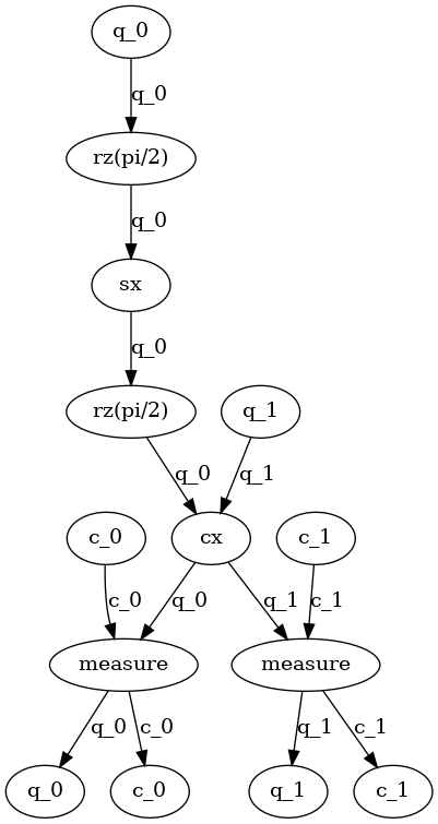
Another example of how the compiler in Qiskit operates on a DAG is to perform analysis to find all the instances of single qubit gates that are executed in series. This series of quantum gates can be analyzed and often simplified into a shorter sequence of gates. A simplified example of this analysis is:

bit_nodes = {"q_0", "q_1", "c_0", "c_1"}

def filter_fn(node):
    # Don't collect input or output nodes
    if node in bit_nodes:
        return False
    # Don't include 2 qubit gates
    if node == "cx":
        return False
    # Ignore non-unitary operations
    if node == "measure":
        return False
    return True

runs = rx.collect_runs(dag, filter_fn)
print(runs)

[['rz(pi/2)', 'sx', 'rz(pi/2)']]

With this we have the DAG nodes that make up a series of 1 qubit gates that we can analyze and attempt to simplify.

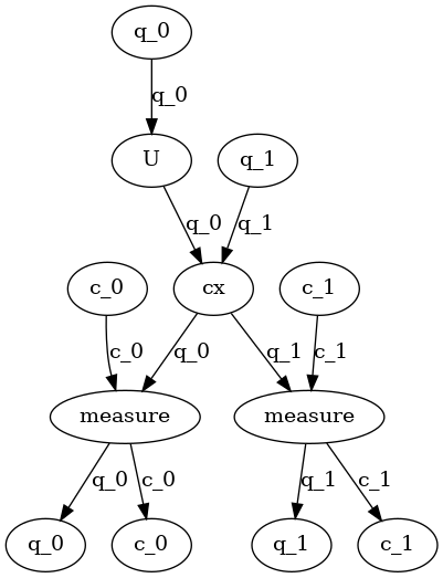
To perform the simplification, we’ll use contract_nodes() to replace a series of nodes (or gates in our case) with a single equivalent node (gate). For example, if the 3 node sequence returned by collect_runs(), ['rz(pi/2)', 'sx', 'rz(pi/2)'], were to be simplified to a single gate "U", it could be done like:

# replace the newest 3 nods (which are the set returned by collect_runs())
dag.contract_nodes(range(len(dag) - 2, len(dag) + 1), "U")
graphviz_draw(
    dag,
    node_attr_fn=lambda node: {"label": str(node)},
    edge_attr_fn=lambda edge: {"label": str(edge)}
)

In Qiskit the node’s index is stored in the node’s data payload, so the above code example is actually written as something like dag.contract_nodes([x._node_id for x in runs[0]], "U"). But this wouldn’t work for the simplified example here.